Model Evaluation Metrics in Machine Learning

You can subscribe to my YouTube channel.

Model evaluation is a core part of building an effective machine-learning model. Model evaluation is very important for any regression and classification algorithm. Based on different evaluation metrics models will be judged and show their real potential.

The idea of model evaluation is to get feedback on the performance of the model. Model building is an iterative process. Building a model then makes model evaluation through different metrics and then improves the model again. This is a cyclic process that keeps on evolving and improves the desired results. Now let’s understand the different metrics for model evaluation.

It is very important to understand the different metrics. Because each metric has its own implication to explain the model performance.

We saw in our previous blog how to build a logistic regression model in Python. let’s use the model to make predictions.

Most of the time we often ask, How accurate is this classification model, Is this model reliable?

To answer these questions we evaluate our model on unseen data with different metrics which will give us enough confidence to support the model. Also using different metrics for evaluation improves the overall predictive power of our model.

Evaluation Metrics

Now, let’s describe the different metrics for classification model evaluation. For Linear Regression Evaluation Metrics check my blog on Model Evaluation Metrics Used For Regression.

Accuracy

Now, the simplest model evaluation metric for classification models is accuracy. you can see the true predicted labels percentage.

In Fig-1 Total of 1406 were predicted correctly as no-churn customers and 298 Churn customers were predicted correctly so,
Accuracy = (1406+298)/(1406+143+263+298) = 0.8076

Accuracy, tells us what proportion of the predictions made by the model is correct. for example, the model is 80.76% accurate, which means a total of 80.76% of the predictions made on the test data are correct.

However, Accuracy does not tell you the whole picture. Even in a model with very high accuracy.

# Splitting the data into train and test
X_train, X_test, y_train, y_test = train_test_split(X,y, train_size=0.7,test_size=0.3,random_state=100)
col = ['PaperlessBilling', 'Contract_One year', 'Contract_Two year',
'PaymentMethod_Electronic check','MultipleLines_No','InternetService_Fiber optic', 
'InternetService_No','OnlineSecurity_Yes','TechSupport_Yes','StreamingMovies_No',
'tenure','TotalCharges']

# Let's run the model using the selected variables
from sklearn.linear_model import LogisticRegression
from sklearn import metrics
logsk = LogisticRegression()
logsk.fit(X_train[col], y_train)

# Making Predictions
# Predicted probabilities
y_pred = logsk.predict_proba(X_test[col])
# Converting y_pred to a dataframe which is an array
y_pred_df = pd.DataFrame(y_pred)
# Converting to column dataframe
y_pred_1 = y_pred_df.iloc[:,[1]]
# Converting y_test to dataframe
y_test_df = pd.DataFrame(y_test)
# Putting CustID to index
y_test_df['CustID'] = y_test_df.index
# Removing index for both dataframes to append them side by side 
y_pred_1.reset_index(drop=True, inplace=True)
y_test_df.reset_index(drop=True, inplace=True)

# Appending y_test_df and y_pred_1
y_pred_final = pd.concat([y_test_df,y_pred_1],axis=1)
# Renaming the column 
y_pred_final= y_pred_final.rename(columns={ 1 : 'Churn_Prob'})
# Rearranging the columns
y_pred_final = y_pred_final.reindex_axis(['CustID','Churn','Churn_Prob'], axis=1)
# Creating new column 'predicted' with 1 if Churn_Prob>0.5 else 0
y_pred_final['predicted'] = y_pred_final.Churn_Prob.map( lambda x: 1 if x > 0.5 else 0)
# Let's see the head
y_pred_final.head()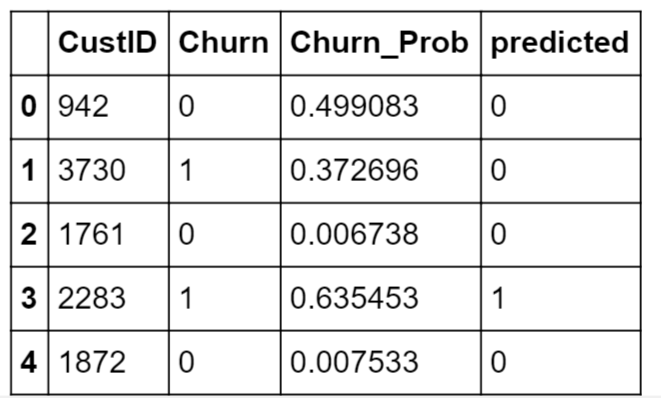

Top 5 predictions of customer churn, now will see how to calculate accuracy using the Sklearn library.

#import library
from sklearn import metrics
# Confusion matrix 
confusion = metrics.confusion_matrix( y_pred_final.Churn, y_pred_final.predicted )
confusion

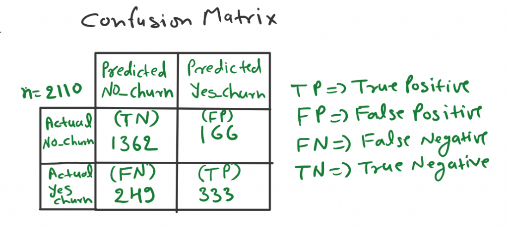
#Let's check the overall accuracy.
metrics.accuracy_score( y_pred_final.Churn, y_pred_final.predicted)
# Accuracy = 0.8033175355450237 which means 80.33%

Accuracy = (1362+333)/(1362+166+249+333) = 0.8033175355450237 which means 80.33%

Confusion Metrix: In the field of machine learning, especially in classification models, a confusion matrix is a specific table that allows visualization of the performance of an algorithm. In Fig-3 we have a confusion matrix of telecom churn data, where the total number of samples is 2110. You can also check the TP, TN, FP, and FN numbers.

Let me give you some understanding of these terms because this is important.

TP (True Positive)

The model predicted positive and it is true. Fig-3 total of 333 observations (People churn) is True positive, which means the model has predicted 333 observations as positive (which means they churn) and it is also true.

TN (True Negative)

The model predicted negative and it is true. Fig-3 the total of 1362 observations is a true negative. This means the model has predicted 1362 observations as negative (People not churn) and it is true.

FP (False Positive)

The model predicted positive but it’s false. Fig-3 a total of 166 observations is a false positive. This means the model has predicted 166 observations as positive (people churn) but not.

FN (False Negative)

The model predicted Negative but it’s False. Fig-3 a total of 249 observations is a false negative. This means the model has predicted 249 observations as Negative (People Not Churn) but it is false (People Really Churn).

Model evaluation Metrics

Now you can see with the help of the confusion matrix we can visualize the performance of the model, now let’s talk about the other model evaluation metrics.

1. Sensitivity
2. Specificity
3. Precision
4. Recall
5. F-1 score

Sensitivity or Recall or TPR (True Positive Rate)

Sensitivity/Recall/ TPR all are the same. and state, that the proportion of actual positive cases which are true.

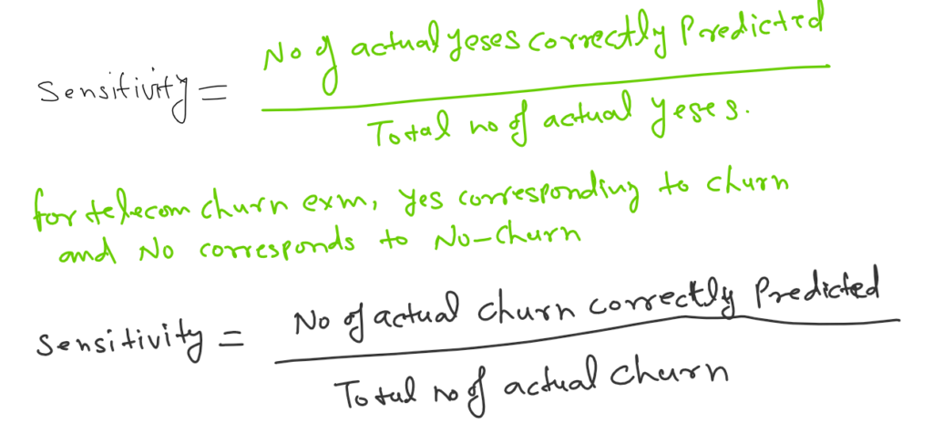
Let me provide you with some signs of Sensitivity metrics.

#Predicted     not_churn    churn
#Actual
#not_churn        1360      168
#churn            249       333  

TP = confusion[1,1] # true positive 
TN = confusion[0,0] # true negatives
FP = confusion[0,1] # false positives
FN = confusion[1,0] # false negatives

#Let's see the sensitivity of our logistic regression model
sensitivity=TP / float(TP+FN)
#0.5721649484536082 or 57.22%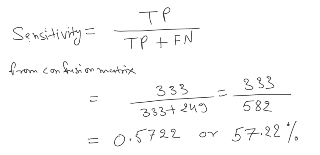

As we can see Sensitivity we are getting only 57%. This means the customer Churn accuracy of the model is 57% which is low accuracy. Before conclusion based on the Sensitivity let me find out the TNR of the model.

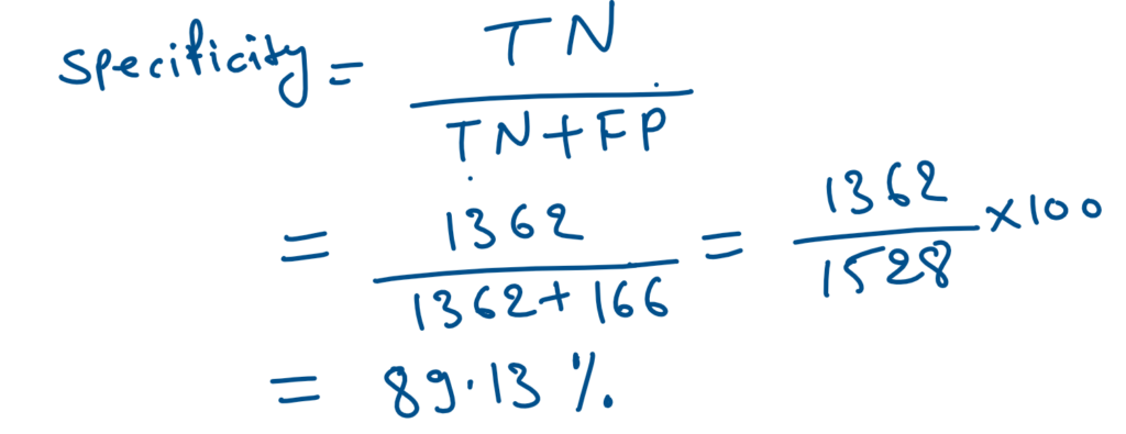
True Negative Rate (TNR) / Specificity

Specificity / TNR are the same. and state, that the proportion of actual negative cases which are true.

# Let us calculate specificity
Specificity = TN / float(TN+FP)
#0.89 or 89%

As we can see above Sensitivity(Churn Accuracy) of the model is 57% and the Specificity(Non-Churn accuracy) of the model is 89%.

NOTE: Now let’s draw some conclusions before moving to another matrix. As we can see the accuracy of the model is very easy to follow. But when we talk about a problem like this where the class distribution is Skewed. In this dataset, as we can see class distribution is not 50-50, rather it’s skewed in nature Non-Churn is 70-75% data and Churn only has 25-30% data. In this kind of dataset, only accuracy is not an important matrix rather Sensitivity and Specificity are more important matrices to evaluate our model.

Let’s deep dive into more details and try to understand the significance of these two matrices in the medical field.

Suppose 1000 people had their COVID-19 tested. (Source)

Out of 427 had positive findings and 573 had negative findings.

Now out of 427 positives who had tested covid positive, 369 of them had an actual COVID-19 positive case.

Out of 573 people who had tested negative for Covid-19, only 558 did not have Covid-19.

Let’s calculate the sensitivity and specificity of the model.

Sensitivity=(True Positives (A))/(True Positives (A)+False Negatives (C))
=(369 (A))/(369(A)+15 (C))
=369/384
Sensitivity=0.961 (Model is predicting 96% level)

Specificity=(True Negatives (D))/(True Negatives (D)+False Positives (B))
Specificity=(558 (D))/(558(D)+58 (B))
Specificity=558/616
Specificity=0.906 (90.6%)

Positive Predictive Value or Precision (PPVs determine, out of all of the positive findings, how many are true positives.)
PPV =(True Positives (A))/(True Positives (A)+False Positives (B))
=(369 (A))/(369 (A)+58(B))
=369/427
PPV =0.864 (86.4%)

Negative Predictive Value (NPVs determine, out of all of the negative findings, how many are true negatives.)
NPV=(True Negatives (D))/(True Negatives (D)+False Negatives(C))
NPV=(558(D))/(558 (D)+15(C))
NPV=(558 )/573
NPV=0.974

Clinical Significance

In this example, I want to explain that Diagnostic testing is a crucial component of evidence-based patient care. If we have a proper understanding of and importance of these matrices. This will help the healthcare provider to understand and make meaningful decisions to improve the patient’s condition.

Now, let’s move to other matrices and find out what we can drive out of those matrices.

Precision

We also call positive predicted value PPVs.

# positive predictive value 
print (TP / float(TP+FP))
# Precision : 0.6646706586826348

Now we will discuss why this is important. We need to think in this way, suppose we have model classes A and B. Class distribution is 97/3 which means 97 data points belong to the A class and 3 data points belong to the B class. We can see there is an imbalance in the class distribution. We can easily build a model with 97% accuracy by saying everything belongs to class A but we need some other matrices that discourage this behavior, we require precision instead of accuracy. That is the reason Precision is important.

ROC Curve.

By plotting the Sensitivity (True positive rate) vs False Positive rate (1-Specificity), we get the Receiver Operating Characteristic (ROC) curve.

A ROC curve demonstrates several things:

1. It shows the tradeoff between sensitivity and specificity (any increase in sensitivity will be accompanied by a decrease in specificity).
2. The closer the curve follows the left-hand border and then the top border of the ROC space, the more accurate the test.
3. The closer the curve comes to the 45-degree diagonal of the ROC space, the less accurate the test.

def draw_roc( actual, probs ):
    fpr, tpr, thresholds = metrics.roc_curve( actual, probs,
                                              drop_intermediate = False )
    auc_score = metrics.roc_auc_score( actual, probs )
    plt.figure(figsize=(6, 4))
    plt.plot( fpr, tpr, label='ROC curve (area = %0.2f)' % auc_score )
    plt.plot([0, 1], [0, 1], 'k--')
    plt.xlim([0.0, 1.0])
    plt.ylim([0.0, 1.05])
    plt.xlabel('False Positive Rate or [1 - True Negative Rate]')
    plt.ylabel('True Positive Rate')
    plt.title('Receiver operating characteristic example')
    plt.legend(loc="lower right")
    plt.show()

    return fpr, tpr, thresholds

draw_roc(y_pred_final.Churn, y_pred_final.predicted)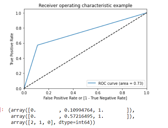

Finding Optimal Cutoff Point
Optimal cutoff probability is that prob where we get balanced sensitivity and specificity

# Let's create columns with different probability cutoffs 
numbers = [float(x)/10 for x in range(10)]
for i in numbers:
    y_pred_final[i]= y_pred_final.Churn_Prob.map( lambda x: 1 if x > i else 0)
y_pred_final.head()

# Now let's calculate accuracy sensitivity and specificity for various probability cutoffs.
cutoff_df = pd.DataFrame( columns = ['prob','accuracy','sensi','speci'])
from sklearn.metrics import confusion_matrix
num = [0.0,0.1,0.2,0.3,0.4,0.5,0.6,0.7,0.8,0.9]
for i in num:
    cm1 = metrics.confusion_matrix( y_pred_final.Churn, y_pred_final[i] )
    total1=sum(sum(cm1))
    accuracy = (cm1[0,0]+cm1[1,1])/total1
    sensi = cm1[0,0]/(cm1[0,0]+cm1[0,1])
    speci = cm1[1,1]/(cm1[1,0]+cm1[1,1])
    cutoff_df.loc[i] =[ i ,accuracy,sensi,speci]
print(cutoff_df)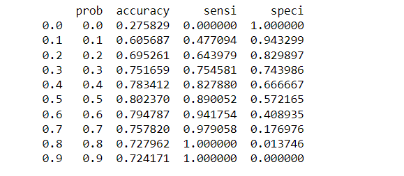

# Let's plot accuracy sensitivity and specificity for various probabilities.
cutoff_df.plot.line(x='prob', y=['accuracy','sensi','speci'])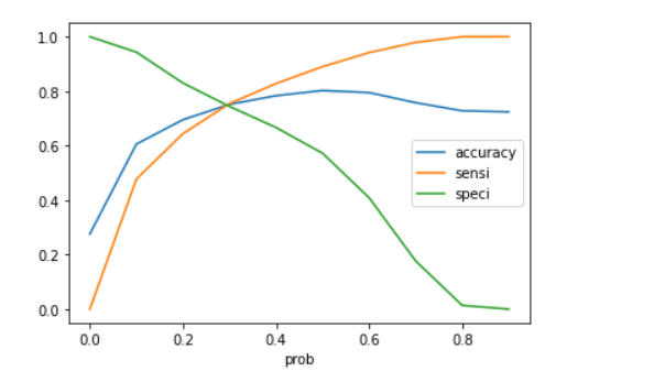

Now we can see from the curve above, 0.3 is the optimum point to take as a cutoff probability. For me covering all the matrics in this blog would be difficult and lengthy to read. so I will add more matrices in a subsequent blog. I will also cover the F1-Score, Log Loss, Gain and Lift Chart, Gini Coefficient, and AUC in a future blog and provide a backlink here.

Footnotes:

Additional Reading

• Logistic Regression for Machine Learning
• Cost Function in Logistic Regression
• Maximum Likelihood Estimation (MLE) for Machine Learning

OK, that’s it, we are done now. If you have any questions or suggestions, please feel free to comment. I’ll come up with more Machine Learning and Data Engineering topics soon. Please also comment and subs if you like my work any suggestions are welcome and appreciated.