An Intuition Behind Gradient Descent using Python

In the last article, we saw the Cost function in detail. Y=β0 + β1x where β0 is the intercept of the fitted line and β1 is the coefficient for the independent variable x. Now the challenges are how we are going to find β0 and β1. β0 intercept and β1 is the slope of the straight line during the training procedure.

In this context, we need to talk about the optimization method which will help us to learn β0 and β1. There are various methods to find an optimal parameter. But in this section will talk about gradient descent which is an iterative method.

As we can see in Fig-1 we have a bunch of data points. Now we want to fit a model (red line), during training, we want to find out optimal β0, β1, and we have an input {Xi, Yi}. So these are our objectives. We will achieve this through an optimization method called Gradient Descent. But before jumping into that we need to find one intermediate step called Cost Function.

To find the best β0, β1, we need to reduce the cost function for all data points.

How to minimize the cost function

There are two types of optimization method

1. Closed-form solution
2. Iterative form solution

Closed-form solution I pretty much covered in my previous blog The Intuition Behind Cost Function. which is nothing but high school Math (Diffraction). How to calculate optimal minima, take a differentiation, and equate to 0

Iterative form solution also has two-part-

1. First Order – also infer to gradient descent
2. Second-Order – Newton Method

So, Gradient descent is an iterative form solution of order one. So to compute optimal thetas, we need to apply Gradient Descent to the Cost function.

Gradient Descent Intution

Gradient descent is one of the most popular algorithms to perform optimization. Gradient descent is an iterative method of optimization of an objective function, in our case the cost function.

Consider a Person (A) in Fig-5 who is walking along the hill below and his destination to reach point B. He can’t view From point A to point B. So the possible action would be either he goes upward or downward. But he might take a bigger step or a little step to reach his destination.

Which way to go and how big a step to take? These are two things that you should know to reach point B.
A gradient descent algorithm will help you to make this decision. now let’s introduce a calculus term called derivative. It is all about slope, the slope of the graph at a particular point. follow this link

Now let’s understand math in the below example. Don’t get confuse β0, β1 is same as θ0, θ1

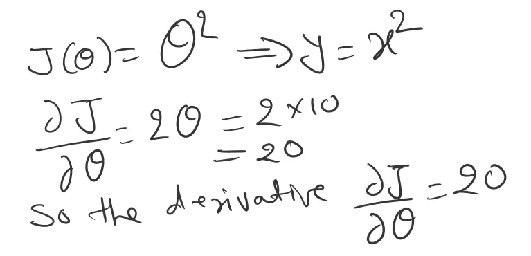
We have function Y=x^2 will start with point θ0=10, now we are going to take a step in a negative direction green direction. Learning rate η = 0.1 and the gradient we have computed as 20, as we can see below.

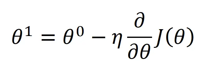
To compute θ1, we saw that the equation will look like this.

Now we have moved in the direction where cost function becoming lesser and we move to position 8. Now if we keep taking these steps we will reach a minimum.

Gradient Descent Formula

The gradient descent formula is:

θ = θ – η * ∇f(θ)

where:

• θ (theta): This represents the parameters of your model that you want to update (e.g., weights and biases in a neural network).
• η (eta): This is the learning rate, a hyperparameter that controls the size of the steps taken during the update process. It determines how much the parameters are adjusted in each iteration based on the error.
• ∇f(θ) (nabla f of theta): This is the gradient of the cost function (f) with respect to the parameters (θ). The gradient tells you the direction of the steepest descent in the cost function’s landscape.

Here’s a breakdown of what the formula does:

1. θ: This represents the current values of your model’s parameters.
2. η * ∇f(θ): This calculates the updated amount based on the learning rate (η) and the gradient (∇f(θ)).
   • Learning rate (η): This determines the step size. A higher learning rate leads to larger steps, potentially reaching the minimum faster but also potentially overshooting it. A lower learning rate leads to smaller steps, ensuring convergence but taking longer.
   • Gradient (∇f(θ)): This points in the direction of the steepest descent of the cost function. By subtracting it from the current parameters (θ), we move the parameters in a direction that will (ideally) decrease the cost function.
3. θ – η * ∇f(θ): This subtracts the updated amount from the current parameters, effectively moving them in the direction that minimizes the cost function.
4. θ (updated): This represents the updated values of the parameters after applying the gradient descent step.

Context

We all are wondering why we are computing with this complex technique. Why we can’t use a Closed-form solution to calculate θ0, and θ1, and reach the solution? Also, we have to choose the η parameter (Learning rate).

So, to understand the context we have a one-dimensional function which is a very easy function. In this case, if you apply gradient descent it will take a lot of effort to reach local minima. We only have to differentiate and equate to zero and will get θ.In 2 dimensions if we differentiate with 2 parameters, θ1,θ2 will get 2 linear equations. We can solve 2 linear equations and get θ1, and θ2 simple.

But if you add more parameters and dimensions. After differentiation, the form of the equation is not linear then we are not able to solve it. So, Closed-form solutions work with simple cases like one or two dimensions. In complex cases, an iterative form solution (Gradient descent) will reach local minima.

To summarize, Though gradient descent looks complicated for a 1-dimension function, it’s easier to compute the optimal minima using gradient descent for higher dimension function. We will be using it in Logistic Regression and even for Neural Networks. 

Learning Rate

So far we have seen, that the gradient is a vector value function. the gradient vector has both a direction and a magnitude. The gradient descent multiplies with η (learning rate) to stimulate the next point.

To compute θ1, as we can see in (Fig-7), the gradient multiplies with η to get the next point.

Now we will understand the intuition for small learning rate vs large learning rate.

• What if η is Big
• What if η is a small

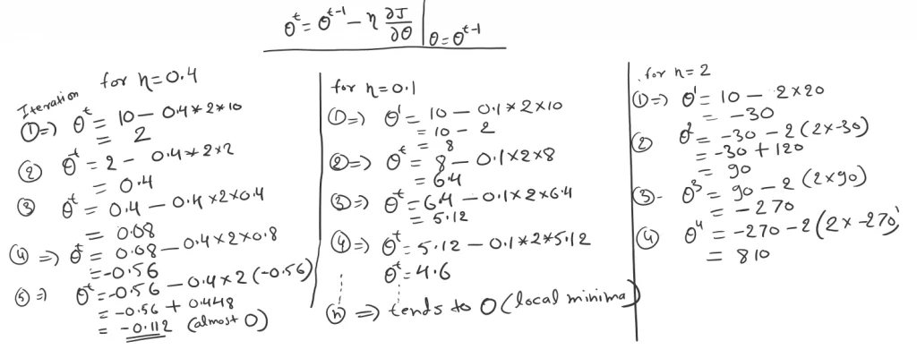
As we can see in Fig-8, we have chosen 3 different learning rates η=0.4, η=0.1, and η=2 respectively.

Observation when η=0.4

When η=0.4 in the first iteration, θ1=2 from 10 to 2 a big jump. And 0.4, 0.8, -0.56, and -0.1 for the 2nd, 3rd, 4th, 5th iterations respectively. So, in the first iteration, it took a long jump but after that, it got conserved and reached local minima. But, if observe on some point we missed the optimal point and do the multiple iterations to reach local minima, overall we can this is a good learning rate to start.

Observation when η=0.1

When η=0.1 As we can see in 1st iteration we reach point 8 from 10, and then to 6.4, 5.12, 4.6, and so on. Which states over the iteration it converges to local minima without oscillating. With this observation, we can say η=0.1 is the best learning rate for this cost function.

Observation when η=2

When η=2 which refers large learning rate as compared to the other two. In the first iteration will get -30 which means starting from 10 to reach -30 point a big jump. Similarly, as we go in each iteration will get 90, -270, and 810 in the 2nd, 3rd, and 4th iterations respectively.
So in a larger learning rate, we could miss the optimal point and Gradient Descent fails to reach the local minimum. As we can see over each iteration θ it becomes larger and diverges to the local minima.

Observation Summary

So the learning rate is a parameter that needs to be adopted as per the problem demands. There would be a situation when η is small then conversion is too slow and when η is large then you could oscillate.

To summarize, A large value of the learning rate may oscillate your solution, and you may skip the optimal solution(global minima). So it’s always a good practice to choose a small value of learning rate and slowly move towards the negative of the gradient.

Gradient Descent in Python

So far we have seen how gradient descent works in terms of the equation. We took a simple 1D and 2D cost function and calculated θ0, θ1, and so on. Followed by multiple iterations to reach an optimal solution.

We will start off by implementing gradient descent for simple linear regression and move forward to perform multiple regression using gradient descent in Python.

Follow the Python code for gradient descent GitHub link with Housing datasets.

# Implement gradient descent function
# Takes in X, y, current m and c (both initialized to 0), num_iterations, learning rate
# returns gradient at current m and c for each pair of m and c
def gradient(X, y, m_current=0, c_current=0, iters=1000, learning_rate=0.01):
    N = float(len(y))
    gd_df = pd.DataFrame( columns = ['m_current', 'c_current','cost'])
    for i in range(iters):
        y_current = (m_current * X) + c_current
        cost = sum([data**2 for data in (y-y_current)]) / N
        m_gradient = -(2/N) * sum(X * (y - y_current))
        c_gradient = -(2/N) * sum(y - y_current)
        m_current = m_current - (learning_rate * m_gradient)
        c_current = c_current - (learning_rate * c_gradient)
        gd_df.loc[i] = [m_current,c_current,cost]
    return(gd_df)

The ‘learning_rate’ variable controls the steps we take in a downward direction in each iteration. If ‘learning_rate’ is too low, the algorithm may take longer to reach the minimum value. On the other hand, if it is high, the algorithm may overstep the minimum value.

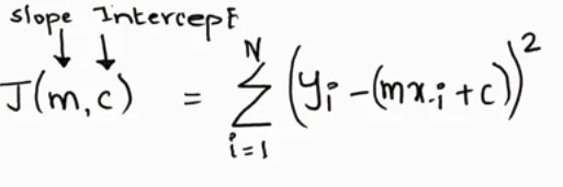
The ‘m_gradient’ variable corresponds to ∂J/∂m, and ‘c_gradient’ corresponds to ∂J/∂c. Moreover, m_current and c_current correspond to the steps in which we are updating the values.

Footnotes:

Gradient descent is an optimization algorithm used to find the values of the parameters. To solve for the gradient, we iterate through our data points using our new m and b values and compute the partial derivatives.

OK, that’s it, we are done now. If you have any questions or suggestions, please feel free to reach out to me. I’ll come up with more Machine Learning topics soon.