Linear Regression is a technique to find the relationship between an independent variable and a dependent variable, Regression is a Parametric machine learning algorithm which means an algorithm can be described and summarize as a learning function.
Example: Y = f(x)
Linear Regression also explains how a change in the dependent variable varies with a unit change of the independent variable. In Simple Linear regression, we can change one variable at a time where else in Multiple Linear regression we can change multiple variables at the same time.
f(x) = Y = B0 + B1*X1 + B2*X2 + B3*X3 (Linear Regression)
Assumptions that are made for linear regression are as follows:
- Linearity
- Outliers
- Autocorrelation
- Multicollinearity
- Heteroskedasticity
Linearity
The relationship between independent and dependent variables must be linear in nature to perform Linear regression if we build a linear model with nonlinear datasets. The model will fail to capture the linear trend mathematically also this will predict wrongly on unseen data.
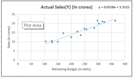
We can create the scatter plot of data to check the linearity and fit the best fit line which fits the given scatter plot in the best way, then we can calculate the residual.
To find the best fit line or regression line we must minimize the cost function.

Residual = |actual value — predicted value| OR


With the above scatter plot we can see the linearity of the data where we can fit the best fit line.
As we can see we start with a scatter plot and we found the best fit line. We also calculated the Residual on each point. The residual sum of squares(RSS) will tell us how to fit our data point on the given regression line.


Outliers
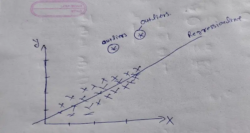
A point that falls outside the data set is called outliers. Which means in statistics an outlier is a data point that significantly differs from the other data points in a sample.

As we can see clearly in the above picture there is two data point significantly different from the other data point.
This will also affect the model if there are good no of outliers best way to split the data set in two-sample and create 2 different model one with outliers and other without outliers.
Outliers also affect the coefficient with changing the sign, Outliers increase the Residual which increases the error.
IQR(Interquartile range) and Box Plot is the technique to identify the outliers.
IQR = Q3-Q1 (where Q3 third quartile, Q1 first quartile)
Data set should be in between this range bellow formula
Outliers range => (Q1–1.5*IQR) to (Q3+ 1.5*IQR)
Multicollinearity
If there is a correlation between predictor variable we can say there is multicollinearity in between. Which mean independent variable are correlated to each other. In the sample, if we found the multicollinearity then it will lead the confusion of the true relationship between dependent and independent variables.
To check for multicollinearity, we can look for the Variance Inflation Factor (VIF) values. A VIF value of 5 or less indicates no multicollinearity.
In high correlation, VIF is >5 and we can drop that variable. Because it would be difficult to estimate the true relation between the dependent and independent variables.
Footnotes:
OK, That’s it, we are done now. If you have any questions or suggestions, please feel free to reach out to me. We will come up with more Machine Learning Algorithms soon.
