Welcome to another blog on Logistic regression in python. In previous blog Logistic Regression for Machine Learning using Python, we saw univariate logistics regression. And we saw basic concepts on Binary classification, Sigmoid Curve, Likelihood function, and Odds and log odds.
In, this section first will take a look at Multivariate Logistic regression concepts. And then we will be building a logistic regression in python.
Logistic Regression for Machine Learning is one of the most popular machine learning algorithms for binary classification.
Multivariate Logistic regression model for Machine Learning
In this logistic regression, multiple variables will use. As we can see there are many variables to classify “Churn”.
For example:
In Multivariate logistic regression, we have multiple independent variable X1, X2, X3, X4,…, Xn. So the expression of Sigmoid function would as bellow.

Telecom Churn use case
So now we will be building a logistic regression model with telecom churn use case.
There is a company ‘X‘ they earn most of the revenue through using voice and internet services. And this company maintains information about the customer.
- Information regarding
- Demographics
- Service Availed
- Expences
There other information they are maintaining and they want to understand customer behavior. They wanted to know whether the customer would churn.
So now lets start and build a model which will tell us whether customer will churn or not. Churn means the customer will switch to other telecom operator.
So, Importing and Merging Data
# Importing Pandas and NumPy
import pandas as pd
import numpy as np
# Importing all datasets
churn_data = pd.read_csv("./churn_data.csv")
customer_data = pd.read_csv("./customer_data.csv")
internet_data = pd.read_csv("./internet_data.csv")So, we have three CSV files. First file churn data which has information related to the customer, Second has customer demographic data. And third, has information related to internet uses of customer.
So we will merge these all three datasets into one single data frame.
#Merging on 'customerID'
df_1 = pd.merge(churn_data, customer_data, how='inner', on='customerID')
#Final dataframe with all predictor variables
telecom = pd.merge(df_1, internet_data, how='inner', on='customerID')
Data Preparation
Now we will perform the data preparation, now convert the categorical variable into 1 or 0.
# Converting Yes to 1 and No to 0
telecom['PhoneService'] = telecom['PhoneService'].map({'Yes': 1, 'No': 0})
telecom['PaperlessBilling'] = telecom['PaperlessBilling'].map({'Yes': 1, 'No': 0})
telecom['Churn'] = telecom['Churn'].map({'Yes': 1, 'No': 0})
telecom['Partner'] = telecom['Partner'].map({'Yes': 1, 'No': 0})
telecom['Dependents'] = telecom['Dependents'].map({'Yes': 1, 'No': 0})
Now will create a dummy variable, In this process we convert categorical variable into dummy/indicator variables. Because Machine learning model only understand the numerical variable. and if we have any categorical variable we can create one-hot-encoding.
Why One-Hot Encode Data in Machine Learning?
A good example of one-hot encoding is categorical variable. But the question is why one-hot encoding is required. Why we can’t fit data directly to model.
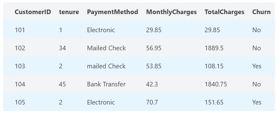
So in a categorical variable from the Table-1 Churn indicator would be ‘Yes’ or ‘No’ which is nothing but a categorical variable. Many machine learning algorithms can’t operate with categorical variables. Because they all required a numerical variable. Only the Decision tree algorithm can work with the categorical variables.
This means the categorical variable must be converted into numeric form. Now we can convert this categorical variable in two ways.
- Numeric encoding
- one-hot encoding
In numerical encoding each unique categorical variable converted into integer value. for example in churn indicator from Table-1 convert into Yes=1 and No=2.
But there is one problem with this numerical encoding use to have an order. Because of this, the model assumes a natural ordering between categories may result in poor performance or unexpected results.
In this case, a one-hot encoding can be applied to the integer representation. This is where the integer encoded variable is removed and a new binary variable is added for each unique integer value.
for example :
Churn indicator has three categorical values Yes, No, Maybe. Therefore three binary variables are needed. A “1” value is placed in the binary variable for the churn and “0” values for the other churn indicator. The binary variables are often called “dummy variables”.
Yes,	No,	Maybe
1,		0,		0
0,		1,		0
0,		0,		1
So, lets go back to our problem, now we will convert all the categorical variable into dummy variable.
# Creating a dummy variable for the variable 'Contract' and dropping the first one.
cont = pd.get_dummies(telecom['Contract'],prefix='Contract',drop_first=True)
#Adding the results to the master dataframe
telecom = pd.concat([telecom,cont],axis=1)
# Creating a dummy variable for the variable 'PaymentMethod' and dropping the first one.
pm = pd.get_dummies(telecom['PaymentMethod'],prefix='PaymentMethod',drop_first=True)
#Adding the results to the master dataframe
telecom = pd.concat([telecom,pm],axis=1)
# Creating a dummy variable for the variable 'gender' and dropping the first one.
gen = pd.get_dummies(telecom['gender'],prefix='gender',drop_first=True)
#Adding the results to the master dataframe
telecom = pd.concat([telecom,gen],axis=1)
# Creating a dummy variable for the variable 'MultipleLines' and dropping the first one.
ml = pd.get_dummies(telecom['MultipleLines'],prefix='MultipleLines')
#  dropping MultipleLines_No phone service column
ml1 = ml.drop(['MultipleLines_No phone service'],1)
#Adding the results to the master dataframe
telecom = pd.concat([telecom,ml1],axis=1)
# Creating a dummy variable for the variable 'InternetService' and dropping the first one.
iser = pd.get_dummies(telecom['InternetService'],prefix='InternetService',drop_first=True)
#Adding the results to the master dataframe
telecom = pd.concat([telecom,iser],axis=1)
# Creating a dummy variable for the variable 'OnlineSecurity'.
os = pd.get_dummies(telecom['OnlineSecurity'],prefix='OnlineSecurity')
os1= os.drop(['OnlineSecurity_No internet service'],1)
#Adding the results to the master dataframe
telecom = pd.concat([telecom,os1],axis=1)
# Creating a dummy variable for the variable 'OnlineBackup'.
ob =pd.get_dummies(telecom['OnlineBackup'],prefix='OnlineBackup')
ob1 =ob.drop(['OnlineBackup_No internet service'],1)
#Adding the results to the master dataframe
telecom = pd.concat([telecom,ob1],axis=1)
# Creating a dummy variable for the variable 'DeviceProtection'.
dp =pd.get_dummies(telecom['DeviceProtection'],prefix='DeviceProtection')
dp1 = dp.drop(['DeviceProtection_No internet service'],1)
#Adding the results to the master dataframe
telecom = pd.concat([telecom,dp1],axis=1)
# Creating a dummy variable for the variable 'TechSupport'.
ts =pd.get_dummies(telecom['TechSupport'],prefix='TechSupport')
ts1 = ts.drop(['TechSupport_No internet service'],1)
#Adding the results to the master dataframe
telecom = pd.concat([telecom,ts1],axis=1)
# Creating a dummy variable for the variable 'StreamingTV'.
st =pd.get_dummies(telecom['StreamingTV'],prefix='StreamingTV')
st1 = st.drop(['StreamingTV_No internet service'],1)
#Adding the results to the master dataframe
telecom = pd.concat([telecom,st1],axis=1)
# Creating a dummy variable for the variable 'StreamingMovies'.
sm =pd.get_dummies(telecom['StreamingMovies'],prefix='StreamingMovies')
sm1 = sm.drop(['StreamingMovies_No internet service'],1)
#Adding the results to the master dataframe
telecom = pd.concat([telecom,sm1],axis=1)
# We have created dummies for the below variables, so we can drop them
telecom = telecom.drop(['Contract','PaymentMethod','gender','MultipleLines','InternetService', 'OnlineSecurity', 'OnlineBackup', 'DeviceProtection',
       'TechSupport', 'StreamingTV', 'StreamingMovies'], 1)
#The varaible was imported as a string we need to convert it to float
telecom['TotalCharges'] =telecom['TotalCharges'].convert_objects(convert_numeric=True)
#telecom['tenure'] = telecom['tenure'].astype(int).astype(float)
Now we can do some cleaning process. Refer this GitHub link
- Checking for outliers in the continuous variables.
- Adding up the missing values column-wise.
- Removing NaN TotalCharges rows
- Normalizing continuous features.
- Standardisation: x=x−mean(x)sd(x)
- (Mean) Normalisation: x=x−min(x)max(x)−min(x) refer this
- Checking the Churn Rate
Model Building
To build the logistic regression model in python. we will use two libraries statsmodels and sklearn. In stats-models, displaying the statistical summary of the model is easier. Such as the significance of coefficients (p-value). and the coefficients themselves, etc., which is not so straightforward in Sklearn.
Let’s start by splitting our data into a training set and a test set.
from sklearn.model_selection import train_test_split
import statsmodels.api as sm
# Putting feature variable to X
X = telecom.drop(['Churn','customerID'],axis=1)
# Putting response variable to y
y = telecom['Churn']
# Splitting the data into train and test
X_train, X_test, y_train, y_test = train_test_split(X,y, train_size=0.7,test_size=0.3,random_state=100)Model-1
# Logistic regression model
logm1 = sm.GLM(y_train,(sm.add_constant(X_train)), family = sm.families.Binomial())
logm1.fit().summary()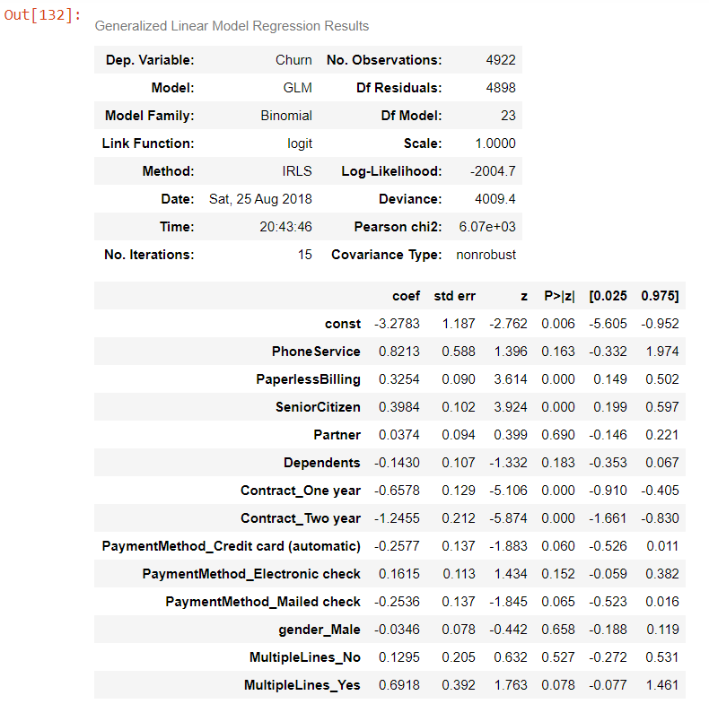
Now if see the correlation metrics
# Importing matplotlib and seaborn
import matplotlib.pyplot as plt
import seaborn as sns
%matplotlib inline
# Let's see the correlation matrix
plt.figure(figsize = (20,10))        # Size of the figure
sns.heatmap(telecom.corr(),annot = True)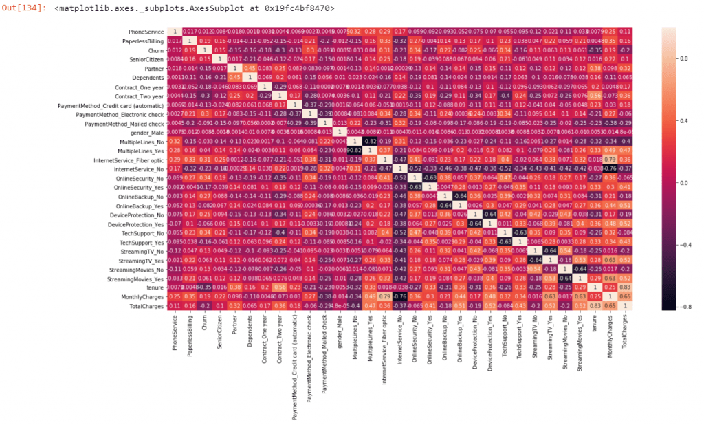
If we found the multicollinearity then it will lead the confusion of the true relationship between dependent and independent variables.
To check for multicollinearity, we can look for the Variance Inflation Factor (VIF) values. A VIF value of 5 or less indicates no multicollinearity. In high correlation, VIF is >5 and we can drop that variable. Because it would be difficult to estimate the true relation between the dependent and independent variables.
So we can see in heat-map lot of variable are highly correlated. So we can drop highly correlated variables.
X_test2 = X_test.drop(['MultipleLines_No','OnlineSecurity_No','OnlineBackup_No','DeviceProtection_No','TechSupport_No','StreamingTV_No','StreamingMovies_No'],1)
X_train2 = X_train.drop(['MultipleLines_No','OnlineSecurity_No','OnlineBackup_No','DeviceProtection_No','TechSupport_No','StreamingTV_No','StreamingMovies_No'],1)
When you have a large number of predictor variables, such as 20-30. It is useful to use an automated feature selection technique such as RFE. To reduce the number of variables to a smaller number (say 10-12) and then manually eliminate a few more.
Feature Selection Using RFE
from sklearn.linear_model import LogisticRegression
logreg = LogisticRegression()
from sklearn.feature_selection import RFE
rfe = RFE(logreg, 13)             # running RFE with 13 variables as output
rfe = rfe.fit(X,y)
print(rfe.support_)           # Printing the boolean results
print(rfe.ranking_)           # Printing the ranking
# Variables selected by RFE
col = ['PhoneService', 'PaperlessBilling', 'Contract_One year', 'Contract_Two year',
'PaymentMethod_Electronic check','MultipleLines_No','InternetService_Fiber optic', 'InternetService_No',
'OnlineSecurity_Yes','TechSupport_Yes','StreamingMovies_No','tenure','TotalCharges']Now Let’s run the model using the selected variables.
# Let's run the model using the selected variables
from sklearn.linear_model import LogisticRegression
from sklearn import metrics
logsk = LogisticRegression()
logsk.fit(X_train[col], y_train)
Model-2
#Comparing the model with StatsModels
logm4 = sm.GLM(y_train,(sm.add_constant(X_train[col])), family = sm.families.Binomial())
logm4.fit().summary()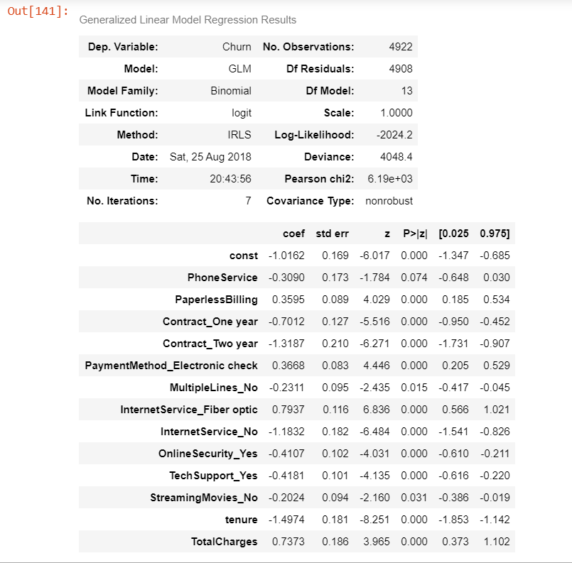
VIF will tell multicollinearity between the independent variable. If VIF > 5, which means a high correlation. Let’s create a method for VIF
# UDF for calculating vif value
def vif_cal(input_data, dependent_col):
    vif_df = pd.DataFrame( columns = ['Var', 'Vif'])
    x_vars=input_data.drop([dependent_col], axis=1)
    xvar_names=x_vars.columns
    for i in range(0,xvar_names.shape[0]):
        y=x_vars[xvar_names[i]]
        x=x_vars[xvar_names.drop(xvar_names[i])]
        rsq=sm.OLS(y,x).fit().rsquared
        vif=round(1/(1-rsq),2)
        vif_df.loc[i] = [xvar_names[i], vif]
    return vif_df.sort_values(by = 'Vif', axis=0, ascending=False, inplace=False)
# Calculating Vif value
vif_cal(input_data=telecom.columns
['PhoneService', 'PaperlessBilling', 'Contract_One year', 'Contract_Two year',
'PaymentMethod_Electronic check','MultipleLines_No','InternetService_Fiber optic', 'InternetService_No',
'OnlineSecurity_Yes','TechSupport_Yes','StreamingMovies_No','tenure','TotalCharges'], dependent_col='Churn')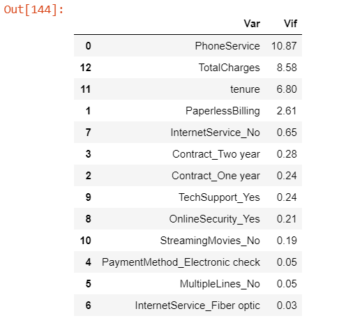
Similarly you can element variable one by one with high VIF value.
Now Let’s run the model using the selected variables using logistic regression. Above we have selected 13 variable now will train the model based on those variable.
# Let's run the model using the selected variables
from sklearn.linear_model import LogisticRegression
from sklearn import metrics
logsk = LogisticRegression()
logsk.fit(X_train[col], y_train)
Making Prediction
# Predicted probabilities
y_pred = logsk.predict_proba(X_test[col])
# Converting y_pred to a dataframe which is an array
y_pred_df = pd.DataFrame(y_pred)
# Converting to column dataframe
y_pred_1 = y_pred_df.iloc[:,[1]]
# Converting y_test to dataframe
y_test_df = pd.DataFrame(y_test)
# Putting CustID to index
y_test_df['CustID'] = y_test_df.index
# Removing index for both dataframes to append them side by side
y_pred_1.reset_index(drop=True, inplace=True)
y_test_df.reset_index(drop=True, inplace=True)
# Appending y_test_df and y_pred_1
y_pred_final = pd.concat([y_test_df,y_pred_1],axis=1)
# Renaming the column
y_pred_final= y_pred_final.rename(columns={ 1 : 'Churn_Prob'})
# Rearranging the columns
y_pred_final = y_pred_final.reindex_axis(['CustID','Churn','Churn_Prob'], axis=1)
# Creating new column 'predicted' with 1 if Churn_Prob>0.5 else 0
y_pred_final['predicted'] = y_pred_final.Churn_Prob.map( lambda x: 1 if x > 0.5 else 0)
# Let's see the head of y_pred_final
y_pred_final.head()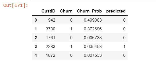
Model Evaluation
from sklearn import metrics
# Confusion matrix
confusion = metrics.confusion_matrix( y_pred_final.Churn, y_pred_final.predicted )
confusion
So let’s check the overall accuracy.
#Let's check the overall accuracy.
acc = metrics.accuracy_score( y_pred_final.Churn, y_pred_final.predicted)
TP = confusion[1,1] # true positive
TN = confusion[0,0] # true negatives
FP = confusion[0,1] # false positives
FN = confusion[1,0] # false negatives
# Let's see the sensitivity of our logistic regression model
Sensitivity = TP / float(TP+FN)
# Let us calculate specificity
Specificity = TN / float(TN+FP)
print('Accuracy : ', acc)
print('Sensitivity ',Sensitivity, ' Specificity ', Specificity)
Accuracy: 0.8033175355450237
Sensitivity: 0.845437616387337
Specificity: 0.6673346693386774
ROC Curve
An ROC curve demonstrates several things:
- It shows the tradeoff between sensitivity and specificity (any increase in sensitivity will be accompanied by a decrease in specificity).
- The closer the curve follows the left-hand border and then the top border of the ROC space, the more accurate the test.
- The closer the curve comes to the 45-degree diagonal of the ROC space, the less accurate the test.
def draw_roc( actual, probs ):
    fpr, tpr, thresholds = metrics.roc_curve( actual, probs,
                                              drop_intermediate = False )
    auc_score = metrics.roc_auc_score( actual, probs )
    plt.figure(figsize=(6, 4))
    plt.plot( fpr, tpr, label='ROC curve (area = %0.2f)' % auc_score )
    plt.plot([0, 1], [0, 1], 'k--')
    plt.xlim([0.0, 1.0])
    plt.ylim([0.0, 1.05])
    plt.xlabel('False Positive Rate or [1 - True Negative Rate]')
    plt.ylabel('True Positive Rate')
    plt.title('Receiver operating characteristic example')
    plt.legend(loc="lower right")
    plt.show()
    return fpr, tpr, thresholds
draw_roc(y_pred_final.Churn, y_pred_final.predicted)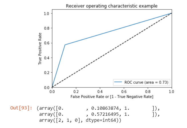
Finding optimal cutoff probability is that prob where we get balanced sensitivity and specificity.
Let’s create columns with different probability cutoffs.
# Let's create columns with different probability cutoffs
numbers = [float(x)/10 for x in range(10)]
for i in numbers:
    y_pred_final[i]= y_pred_final.Churn_Prob.map( lambda x: 1 if x > i else 0)
y_pred_final.head()
Now let’s calculate accuracy sensitivity and specificity for various probability cutoffs.
# Now let's calculate accuracy sensitivity and specificity for various probability cutoffs.
cutoff_df = pd.DataFrame( columns = ['prob','accuracy','sensi','speci'])
from sklearn.metrics import confusion_matrix
num = [0.0,0.1,0.2,0.3,0.4,0.5,0.6,0.7,0.8,0.9]
for i in num:
    cm1 = metrics.confusion_matrix( y_pred_final.Churn, y_pred_final[i] )
    total1=sum(sum(cm1))
    accuracy = (cm1[0,0]+cm1[1,1])/total1
    sensi = cm1[0,0]/(cm1[0,0]+cm1[0,1])
    speci = cm1[1,1]/(cm1[1,0]+cm1[1,1])
    cutoff_df.loc[i] =[ i ,accuracy,sensi,speci]
print(cutoff_df)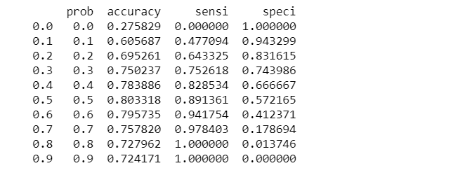
Let’s plot accuracy sensitivity and specificity for various probabilities.
# Let's plot accuracy sensitivity and specificity for various probabilities.
cutoff_df.plot.line(x='prob', y=['accuracy','sensi','speci'])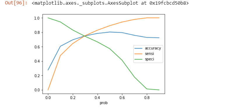
From the curve above, 0.3 is the optimum point to take as a cutoff probability.
y_pred_final['final_predicted'] = y_pred_final.Churn_Prob.map( lambda x: 1 if x > 0.3 else 0)
#Let's check the overall accuracy.
metrics.accuracy_score( y_pred_final.Churn, y_pred_final.final_predicted)
Model Accuracy : 0.7502369668246446
You can find the full code implementation on my GitHub.
Classification accuracy will be used to evaluate each model. After all of this was done, a logistic regression model was built in Python using the function glm() under statsmodel library. This model contained all the variables, some of which had insignificant coefficients; for many of them, the coefficients were NA. Hence, some of these variables were removed based on VIF and p-value.
Footnotes:
Additional Reading
- Logistic Regression for Machine Learning
- Cost Function in Logistic Regression
- Maximum Likelihood Estimation (MLE) for Machine Learning
OK, that’s it, we are done now. If you have any questions or suggestions, please feel free to comment. I’ll come up with more Machine Learning topic soon.

Can you please explain how you have found out that there is no outliers?
To identify outlier, you can use either box plot to view the distribution or identify outliers with interquartile range. In our case if you take a look on dictionary file (definition of all column) check this (https://github.com/brijesh1100/LogisticRegression/blob/master/Multivariate/Telecom%20Churn%20Data%20Dictionary.csv) Tenure: The time for which a customer has been using the service. TotalCharges : The total money paid by the customer to the company. I have taken interquartile range from 25% to 99% range and as you increase the tenure your total charges will increase. and you can clearly see the distribution range of 25 to 99 there is no sudden spike in… Read more »
Okay, I understood what you are trying to say. I was following some different way to find out the outlier using Interquartile range. I am attaching the snip of that. Also, I am sharing the link: Medium article. I am just not sure how to use this in our case.