Model Evaluation Metrics Used For Regression.

The regression model works on the constructive evaluation principle. We build a model, check from metrics, and then make improvements. And continue until we achieve a desirable accuracy. Evaluation metrics explain the performance of a model.

Model evaluation used in all types of algorithms Linear Regression

Evaluation metrics

• R-Squared
• Adjusted R-Squared
• RMSE
• VIF
• P-Value
• Residual.

R-Squared

R-squared is an evaluation metric. Through this, we can measure, how good the model is higher the R-square better the accuracy.

For example:

Let’s say after evaluation we got R-squared = 0.81. This means we can explain 81% of the variance in data, also we can say the accuracy of a model is 81%.

We can compute the RSS (Residual sum squared) with the square sum of (actual — predicted).

In TSS (Total sum squared) we need to take the squared sum of (predicted — mean value)

R2 = 1, Residual is 0 and R-Squared = 1

Best fit, as you can see as the fit line getting poor the R-Squared value. Also, gets reduced and becomes close to zero R-squared lies between 0 to 1

0 < R-Squared <=1

Model-1

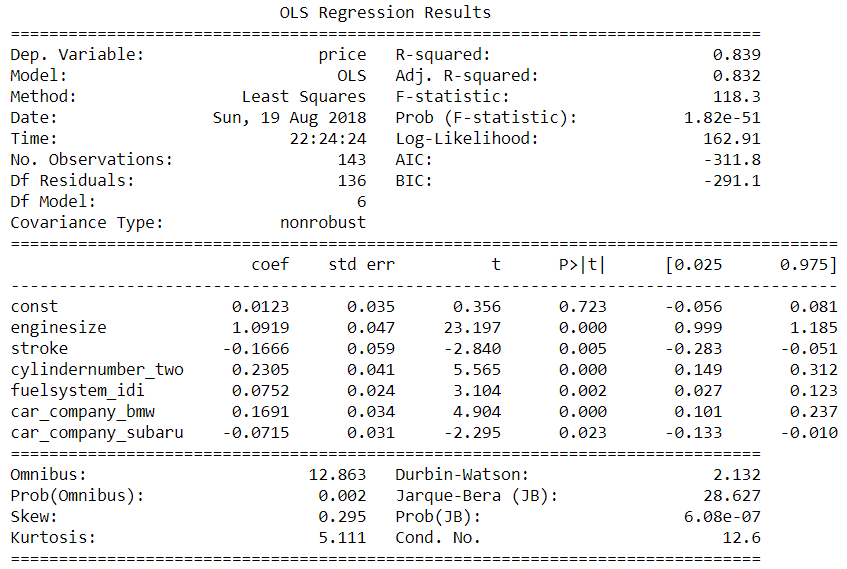
As you can see in the final model we got R-squared = 0.839

This means we can explain 83% of the variance in data, also we can say the accuracy of a model is 83%.

Adjusted R-Squared:

Adjusted R-Squared Penalize the model that has too many features or variables.

Let’s say we have 2 models each with 3 features R-squared is 83.9% and adjusted-R-Squared 83.2%

Now if we add 3 more features in the first model R-Squared will get an increase. But adjusted-R-Squared will penalize the model. It will tell you I am giving you a lower value as you have added a new feature which could be because of a problem in modeling.

The adjusted R-squared increases only if the new term improves in the model. Adjusted R-squared gives the percentage of variation explained by only those independent variables. That affects the dependent variable. Adjusted R-squared also measures the goodness of the model.

As we can see in our final Model-1 R-squared and adjusted R-squared are very close.

R-Squared = 0.839

Adjusted R-Squared =0.832.

With this, we assume none of the other variables need to be added to the model as a predictor.

P-Value and VIF

The P-value will tell us how significant the variable is. And VIF will tell multicollinearity between the independent variable. If VIF > 5, it means a high correlation.

The P-value will tell the probability of the accepted Null Hypothesis. Which means the probability of failing to reject the Null Hypothesis.

The higher the P-value higher the probability of failure to reject a Null Hypothesis.

The lower the P-value higher the probability that the Null Hypothesis will be rejected.

Our Observation is if we see the above final model. All variable has less the 0.05 P-value. Which means they are highly significant variables.

VIF value is less than 5 in our final model. We can say there is no correlation between the independent variable.

RMSE: (Root Mean Square)

The most popular used metric is RMSE. This will measure the differences between sample values predicted, and the values observed. Because Root Mean Square Error (RMSE) is a standard way to measure the error of a model in predicting quantitative data.

The RMSE is the standard deviation of the residuals (prediction errors). Residuals are a measure of how far from the regression line data points are.

It will evaluate the sum of mean squared error over the number of total sample observations.

In Model-1 we calculated the RMSE: 0.08586514469292264. Lowering the RMSE better the model performance.

Durbin-Watson: The Durbin-Watson test evaluates the Autocorrelation it should lie between 0 to 4

In our above observation in the final model, we got Durbin-Watson: 2.132

Summary:

There are some disadvantages if we do not consider our evaluation metrics, which will increase the in-performance measurement. For all metrics, R-squared, Adjusted R-squared, RMSE, VIF, P-Value, Residual, and Durbin-Watson, Will tell us how good the model is (best-fit model) each metric is important for model evaluation as I describe above.

In Linear Regression there are some assumptions:

1. Linearity
2. Outliers
3. Autocorrelation
4. Multicollinearity
5. Heteroskedasticity

which we need to check while measuring the metrics.

• RMASE has a disadvantage RMSE will be affected by the outliers. If we have outliers in our data sample
• If the sample population is not linear RMSE will be affected as there would be no trend which means standard division will vary.
• Residual is also affected by the outliers which will increase the residual squared sum.

stroke, engine size, fuelsystem_idi, car_company_bmw, cylindernumber_two, car_company_subaru

These are the driving factors as per the Model-1 on which the pricing of cars depends.

Observation

• I can see a good model with R-Square = 0.839
• I can see good-adjusted R-squared = 0.832
• As R-squared and adjusted R-squared are very close, we can assume none of the other variables need to be added to the model as a predictor.
• The model has Durbin-Watson:2.132 which is between 0 and 4, we can assume there is no Autocorrelation
• As we can see VIF<5 which means no Multicollinearity
• P-value is less than 0.05 which means they are highly significant variables.

Footnotes

If you have any questions or suggestions, please feel free to reach out to me. I’ll come up with more Machine Learning topics soon.